The {soccerAnimate} R package just received a significant update, offering new functionalities for analyzing and visualizing individual player performance and team average positioning. This update caters to football analysts who primarily use R for their data exploration.
In case you are interested to check the package functionalities from the beginning, start looking at this previous blogpost.
Let’s share some details about these new features in the following article.
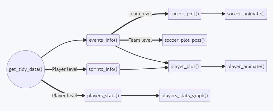
First of all, consider this diagram as a general guideline for the functions of the package:
1) In-Depth Player Analysis
Inspired by the Laurie Shaw’s Youtube video on extracting insights from tracking data, this update provides R alternatives to Python functionality. Now you can calculate valuable player statistics like:
Minutes played and average speed
Instantaneous velocity (magnitude and direction) to derive game-level stats and visualizations
Total distances covered throughout the game and within specific speed ranges (you are able to choose between 2 kind of ranges)
Number of sprints made by each player
Visualizing Player Performance:
Visualizations are key to understanding player movement. The update offers functions to create:
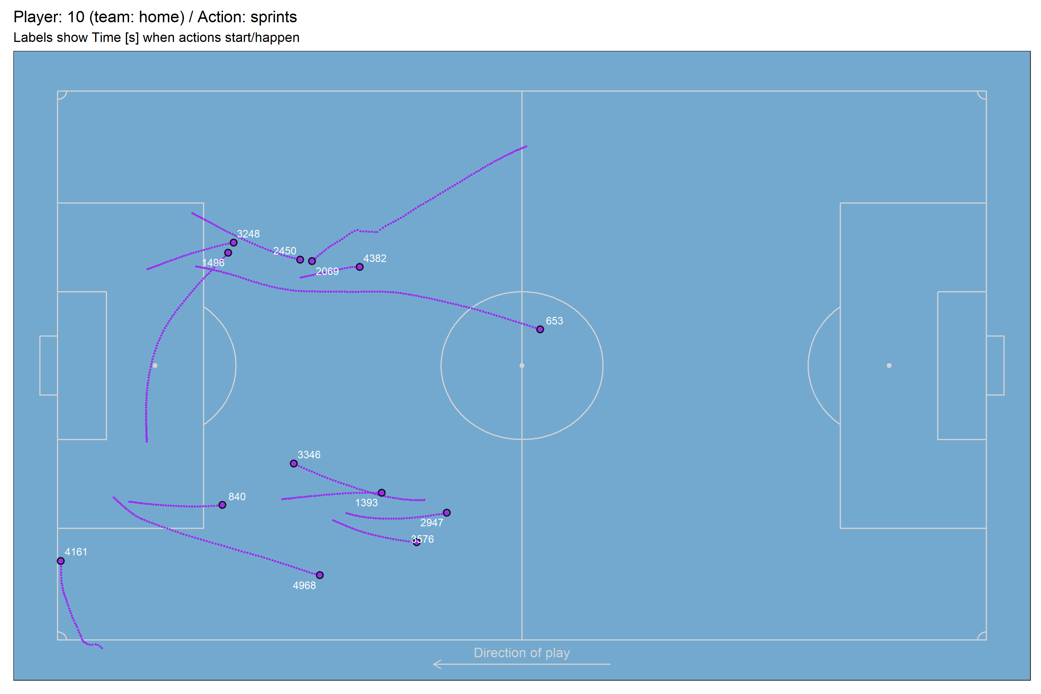
Plots showing a specific player’s actions (e.g., sprints) on the field
Animations highlighting player paths throughout a specific timeframe
Example 1
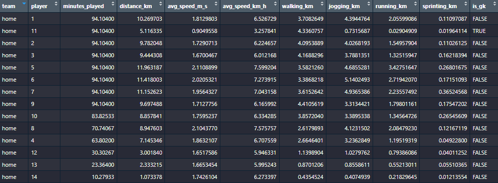
With the function players_stats() you calculate for every player on a specific game, their respective minutes played, avg. speed, total distance and distance for different speed ranges.
Then you are able to visualize those stats with the function players_stats_graph() (Home team by default):
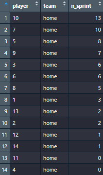
With the function sprints_info() you apply the needed data processing to get the number of sprints that every player for a chosen team (Home team by default) made over a specific game. A sprint is considered when a player run a very high speed (higher than 7 [m/s]) for at least 1 second.
With this information you can observe a player ranking based on the number of sprints:
And finally, with the function player_animate() you are able to create a 2D animation for the specific time range when one specific player sprint happened.
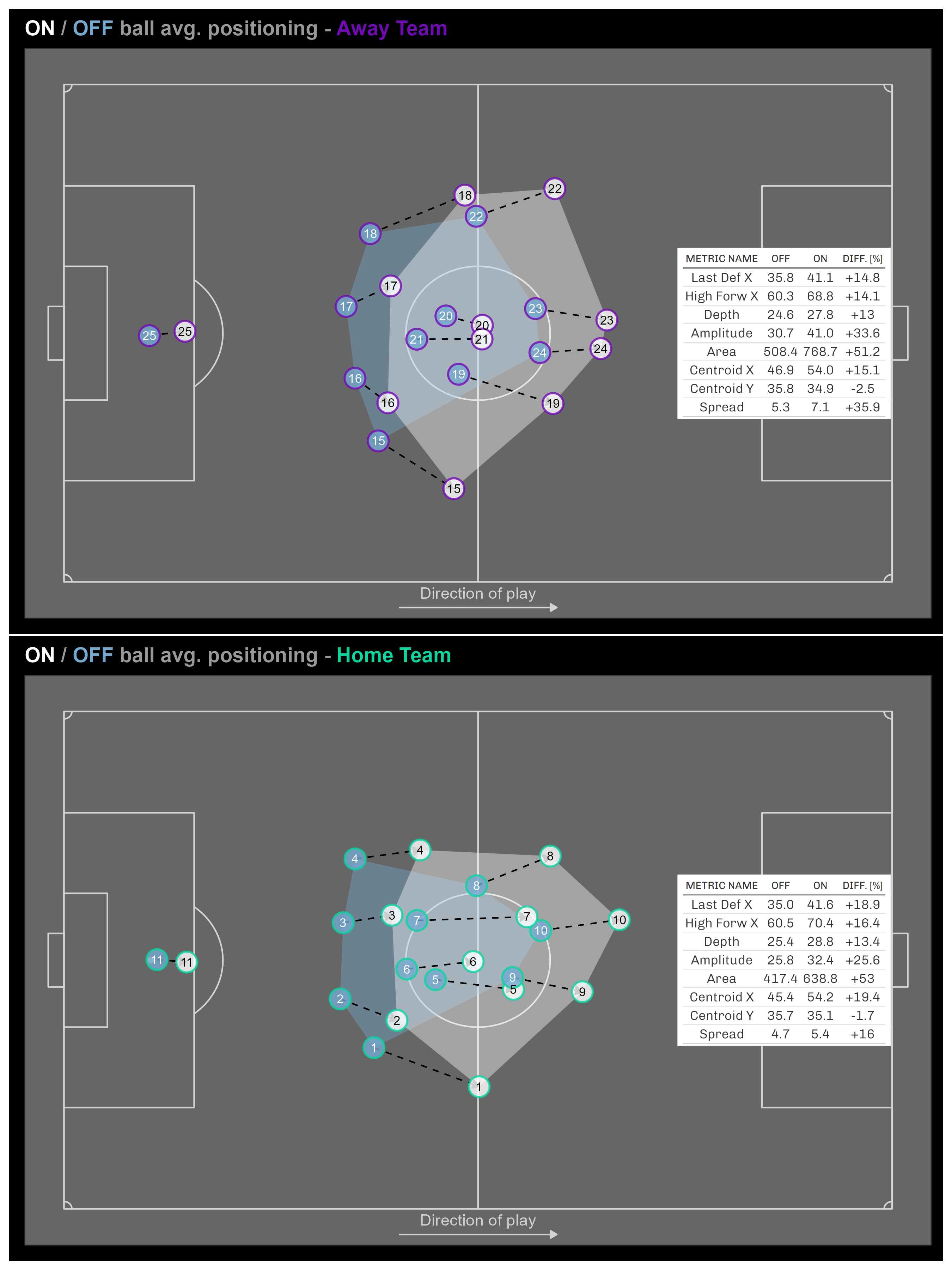
The update also adds functionalities for analyzing team positioning:
Visualizations comparing team average positions during ON and OFF ball possession states
Average positioning statistics for the team including:
Lowest defender X position [m]
Highest forward X position [m]
Depth [m]
Amplitude [m]
Area [m2]
Centroid X,Y
Spread
Additionally, you can see the percentage change in these stats between ON and OFF ball possession for each team.
Example 3
With the function soccer_plot_poss() you can create a plot showing for each team the avg. position of players, its convex hull and respective position stats.
Show code
event_path ="https://raw.githubusercontent.com/metrica-sports/sample-data/master/data/Sample_Game_2/Sample_Game_2_RawEventsData.csv"soccer_plot_poss(td, event_path, team ="Away", pitch_fill ="grey40",on_ball_col ="white", off_ball_col ="#74a9cf")
The Road Ahead
As you can note, now a better understanding of the physical players performance over a specific game can be obtained in addition to a more complete idea about the team avg. position (and shape) between ON & OFF ball possession states.
Future updates for {soccerAnimate} could include:
New visualizations and statistics for target team possession vs. opponent off possession scenarios
Splitting stats and positioning by context (score, venue, game state, etc.)
Adding specific metric annotations to visualizations
Supporting data providers beyond Metrica Sports
I’m excited about these enhancements and hope they empower you to delve deeper into football data analysis with R! Stay tuned for further updates on the {soccerAnimate} package.